smartcor detects variable types and selects a suitable correlation method for each pair. It supports continuous, count, binary, ordinal, and categorical variables and returns the estimate, inference, selected method, and rationale. The package is available in two languages, kept at feature parity: smartcor for R, on CRAN, and pysmartcor for Python, on PyPI.
Version 1.2.0
Version 1.2.0 follows the decision framework of the accompanying paper. Before choosing a method, smart_cor() now checks each pair for outliers (outer fences), normality (Mardia or Jarque-Bera), latent normality (the LR test of the threshold model), and linearity. The default method changes for eight of the ten variable-type pairs, and four estimators are new: biserial, the correlation ratio eta-squared, Kruskal-Wallis eta-squared, and Freeman’s theta. Read the decision framework for the rules and the changelog for the full list of changes.
nearPD remains off by default. Enable it explicitly with nearPD = TRUE in R or nearPD=True in Python. Original pairwise estimates and inference remain available through smart_cormat().
The examples below use version 1.2.0.
Installation
Install the R package from CRAN:
install.packages("smartcor")Install the Python package from PyPI:
The two implementations share the same decision logic, estimators, and inference; see smartcor in Python for the full R-to-Python translation table.
Quick start in R
The package bundles a frozen extract of the 2024 General Social Survey, used in all examples.
library(smartcor)

csv = system.file("extdata", "gss_2024_casestudy.csv", package = "smartcor")
gss = read.csv(csv)
Correlate one pair and get the estimate, the selected method, the diagnostics, and the reasoning:
result = smart_cor(gss$coninc, gss$sex, verbose = FALSE)
print(result)
#>
#> ── Smart Correlation ───────────────────────────────────────────────────────────
#> Estimate: -0.1336
#> Method: Rank-Biserial Correlation
#> Variables: gss$coninc ("continuous") × gss$sex ("binary")
#> N: 3000
#> p-value: < 0.001
#> Test: Wald test on Fisher-z scale
#> H0: delta = 0
#> Small p-values (e.g., p < 0.05) indicate evidence against H0.
#> 95% CI: [-0.1743, -0.0925]
#> Source: Cliff (1996)
#>
#> Diagnostics
#> Outliers (outer fence): none
#> Normality (Jarque-Bera): p < 2e-16 (rejected)
#>
#> The Jarque-Bera test rejects normality of the within-group residuals (p <
#> 2e-16); Rank-Biserial Correlation selected.
#>
#> ℹ Alternatives: "point_biserial" and "biserial" (pass `method = "..."` to use)
Build a matrix across mixed variable types:
columns = c("age", "coninc", "degree", "happy", "sex", "region")
matrix = smart_cormat(gss[, columns], seed = 1, verbose = FALSE)

round(matrix$correlations, 3)
#>           age coninc degree  happy    sex region
#> age     1.000  0.037  0.021 -0.046 -0.010  0.008
#> coninc  0.037  1.000  0.357 -0.136 -0.134  0.019
#> degree  0.021  0.357  1.000 -0.079  0.015  0.043
#> happy  -0.046 -0.136 -0.079  1.000 -0.007  0.027
#> sex    -0.010 -0.134  0.015 -0.007  1.000  0.063
#> region  0.008  0.019  0.043  0.027  0.063  1.000
matrix$methods
#>        age              coninc           degree           happy
#> age    "pearson"        "spearman"       "kendall"        "kendall"
#> coninc "spearman"       "pearson"        "kendall"        "kendall"
#> degree "kendall"        "kendall"        "polychoric"     "kendall"
#> happy  "kendall"        "kendall"        "kendall"        "polychoric"
#> sex    "rank_biserial"  "rank_biserial"  "rank_biserial"  "polychoric"
#> region "kw_eta_squared" "kw_eta_squared" "freemans_theta" "freemans_theta"
#>        sex             region
#> age    "rank_biserial" "kw_eta_squared"
#> coninc "rank_biserial" "kw_eta_squared"
#> degree "rank_biserial" "freemans_theta"
#> happy  "polychoric"    "freemans_theta"
#> sex    "phi"           "cramers_v"
#> region "cramers_v"     "cramers_v"
Plot it:
ggcor_heatmap(matrix)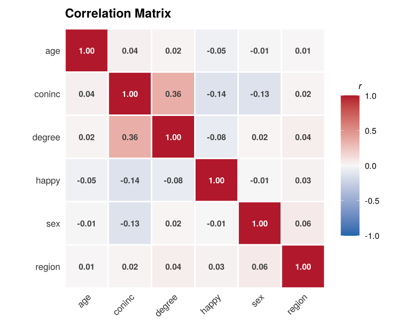
plot of chunk heatmap
Quick start in Python
The same workflow in Python, with the same bundled data:
from importlib.resources import as_file, files

import pandas as pd

from pysmartcor import smart_cor, smart_cormat

with as_file(files("pysmartcor").joinpath("data/gss_2024_casestudy.csv")) as csv:
    gss = pd.read_csv(csv)

result = smart_cor(gss["coninc"], gss["sex"], verbose=False)
print(result)
Inspect result.method, result.rationale, and result.diagnostics for the selection and the tests behind it.
Methods
The package implements 18 methods and selects among them as follows:
| Variable types | Default method | Alternative |
|---|---|---|
| Correlation methods (signed, from -1 to +1) | ||
| Continuous + continuous | Pearson (linear, no outliers) | Spearman (outliers or nonlinear), Kendall’s tau |
| Continuous + binary | Biserial (if latent normality holds) | Point-biserial; rank-biserial (outliers or non-normal) |
| Binary + binary | Pearson = phi | Tetrachoric (latent normal), Yule’s Q (no latent continuum) |
| Continuous + ordinal | Polyserial (if latent normality holds) | Kendall’s tau (m <= 5) or Spearman |
| Ordinal + ordinal | Polychoric (if latent normality holds) | Kendall’s tau (m <= 5) or Spearman; Goodman-Kruskal gamma |
| Binary + ordinal | Polychoric (if latent normality holds) | Rank-biserial; Kendall’s tau, Spearman |
| Association measures (unsigned, from 0 to 1) | ||
| Continuous + categorical | Correlation ratio eta-squared | Kruskal-Wallis eta-squared (outliers or non-normal); Cramer’s V (binned) |
| Binary + categorical | Cramer’s V | – |
| Ordinal + categorical | Freeman’s theta | Cramer’s V |
| Categorical + categorical | Cramer’s V | Theil’s U, Tschuprow’s T |
m is the number of categories of the ordinal variable (the smaller of the two for an ordinal pair). Count variables follow the continuous rows. Each method comes with a confidence interval and a p-value.
Paper
The accompanying paper, smartcor: Intelligent Correlation Method Selection for Mixed Variable Types by M. Harshvardhan and Pritam Ranjan (2026), is available as an arXiv preprint: arXiv:2607.22285 (doi:10.48550/arXiv.2607.22285). The package vignettes cover the same material: method selection, the underlying theory, and inference.